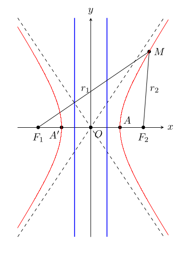
TikZ will normally plot from -5 to 5. If you want to use a different plotting interval, you will have to somehow communicate this to TikZ. 

To simplify the code a bit, you could set the domain globally for the whole tikzpicture, so you don't have to repeat it for every plot:

```
\documentclass[tikz,border=3mm]{standalone}
\usepackage{calc}
\begin{document}
	\begin{tikzpicture}[>=stealth,domain=-1.6:1.6]
	\pgfmathsetmacro{\e}{1.8}   % eccentricity
	\pgfmathsetmacro{\a}{1}
	\pgfmathsetmacro{\b}{(\a*sqrt((\e)^2-1)} 
	\pgfmathsetmacro{\c}{sqrt(\a^2+\b^2)} 
	\pgfmathsetmacro{\k}{1.5}
	\pgfmathsetmacro{\xmin}{-\a-\k}
	\pgfmathsetmacro{\xmax}{\a+\k}
	\draw[red] plot ({\a*cosh(\x)},{\b*sinh(\x)});
	\draw[red] plot ({-\a*cosh(\x)},{\b*sinh(\x)});
	\path 
	(-\c,0) coordinate (F_1)
	(\c,0) coordinate (F_2)
	(0,0) coordinate (O)
	(-\a,0) coordinate (A')
	(\a,0) coordinate (A)
	({\a*sec(60)},{\b*tan(60)}) coordinate (M) 
	;
	\draw[->] (\xmin,0) -- (\xmax,0) node[right]{$x$};
	\draw[ ->] (0,\b/\a*\xmin) -- (0,\b/\a*\xmax) node[above]{$y$};
	\draw[dashed, domain=\xmin:\xmax] plot(\x,{\b/\a*\x});
	\draw[dashed, domain=\xmin:\xmax] plot(\x,{-\b/\a*\x});
	\draw[thick, blue](\a/\e,\b/\a*\xmin) -- (\a/\e,\b/\a*\xmax);
	\draw[thick, blue] (-\a/\e,\b/\a*\xmin) -- (-\a/\e,\b/\a*\xmax);
	\foreach \p in {A,A',O,F_1,F_2,M}
	\draw[fill=black] (\p) circle (1.5pt);
	\foreach \p/\g in {A/45,A'/-135,O/-40,F_1/-90,F_2/-90,M/0}
	\path (\p)+(\g:3.5mm) node{$\p$};	
	\draw (F_1) -- (M) node[midway,left]{$ r_1 $};
	\draw (F_2) -- (M) node[midway, right]{$ r_2 $};
\end{tikzpicture}

\end{document}
```

If you don't exactly need your plot to go from -1.6 to 1.6, but just to be within your axis, you could clip the graph (this will be considerable slower and needs more samples as the whole graph needs to be calculated):

```
\documentclass[tikz,border=6mm]{standalone}
\usepackage{calc}
\begin{document}
	\begin{tikzpicture}[>=stealth]
	\pgfmathsetmacro{\e}{1.8}   % eccentricity
	\pgfmathsetmacro{\a}{1}
	\pgfmathsetmacro{\b}{(\a*sqrt((\e)^2-1)} 
	\pgfmathsetmacro{\c}{sqrt(\a^2+\b^2)} 
	\pgfmathsetmacro{\k}{1.5}
	\pgfmathsetmacro{\xmin}{-\a-\k}
	\pgfmathsetmacro{\xmax}{\a+\k}
	\path 
	(-\c,0) coordinate (F_1)
	(\c,0) coordinate (F_2)
	(0,0) coordinate (O)
	(-\a,0) coordinate (A')
	(\a,0) coordinate (A)
	({\a*sec(60)},{\b*tan(60)}) coordinate (M) 
	;
	\draw[->] (\xmin,0) -- (\xmax,0) node[right,overlay]{$x$};
	\draw[ ->] (0,\b/\a*\xmin) -- (0,\b/\a*\xmax) node[above,overlay]{$y$};
	\draw[dashed, domain=\xmin:\xmax] plot(\x,{\b/\a*\x});
	\draw[dashed, domain=\xmin:\xmax] plot(\x,{-\b/\a*\x});
	\draw[thick, blue](\a/\e,\b/\a*\xmin) -- (\a/\e,\b/\a*\xmax);
	\draw[thick, blue] (-\a/\e,\b/\a*\xmin) -- (-\a/\e,\b/\a*\xmax);
	\foreach \p in {A,A',O,F_1,F_2,M}
	\draw[fill=black] (\p) circle (1.5pt);
	\foreach \p/\g in {A/45,A'/-135,O/-40,F_1/-90,F_2/-90,M/0}
	\path (\p)+(\g:3.5mm) node{$\p$};	
	\draw (F_1) -- (M) node[midway,left]{$ r_1 $};
	\draw (F_2) -- (M) node[midway, right]{$ r_2 $};
  \begin{scope}
    \clip (current bounding box.south west) rectangle (current bounding box.north east);
  	\draw[red,samples=2000] plot ({\a*cosh(\x)},{\b*sinh(\x)});
  	\draw[red,samples=2000] plot ({-\a*cosh(\x)},{\b*sinh(\x)});
  \end{scope}
\end{tikzpicture}

\end{document}
```

![document-1.png](/image?hash=c93093ea94542017c88b4816730a949e61628a334945133cb05df53973bb2d72)