JeT

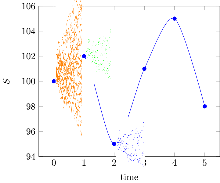
I'd like to replace the mark of my plot with a mini brownian diffusion.
I'll probably need to embed it in a `pic`.
I have the ingredients, I need a little help (some would say I am missing a pi(e)c(e)... ) on the recipe.
I don't look for the version below with one brownian replicated 5 times and not consistent with the measure on the main graph.
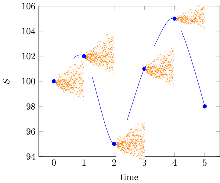
I imagine more something like (Poorly copied pasted) with one brownian per period, whose coordinates are consistent with the main plot.
**Where do I need help ?**
I'd like each brownian
- to start at the mark
- have a width of one tick for the pic
- diffusion being consistent with the main plot grid
Details in the MWE below.
```
\documentclass[tikz]{standalone}
\usepackage{pgfplots, pgfplotstable}
\usetikzlibrary{positioning}
\tikzset{
declare function={
invgauss(\a,\b) = sqrt(-2*ln(\a))*cos(deg(2*pi*\b));
}
}
%-----------------------------------------------------------------
% Code from Jake @ TeX.SE to generate brownian motions
% If you have an idea to load to improve the compilation time
\makeatletter
\pgfplotsset{
table/.cd,
brownian motion/.style={
create on use/brown/.style={
create col/expr accum={
(\coordindex>0)*(
max(
min(
invgauss(rnd,rnd)*0.25*sqrt(1)+\pgfmathaccuma,
\pgfplots@brownian@max
),
\pgfplots@brownian@min
)
) + (\coordindex<1)*\pgfplots@brownian@start
}{\pgfplots@brownian@start}
},
y=brown, x expr={\coordindex},
brownian motion/.cd,
#1,
/.cd
},
brownian motion/.cd,
min/.store in=\pgfplots@brownian@min,
min=-inf,
max/.store in=\pgfplots@brownian@max,
max=inf,
start/.store in=\pgfplots@brownian@start,
start= 0
}
\makeatother
%-----------------------------------------------------------------
% Create the pic that generates brownian motions
% I did my homework and read the pgfmanual.
% It enabled me to use parameters in `pic`
% The idea is to have flexibility on the brownian
% \pic{BM=color/Starting@y/nbs of paths/nbs of points in the path};
% "nbs of points in the path" represents the subdivision of 1 unit of time
\tikzset{pics/BM/.style args={#1/#2/#3/#4}{
code = {%
\pgfmathsetseed{3}
\pgfplotstablenew{#4}\wiener % Initialise an empty table with #4 steps for brownians
\node[](#1){
\begin{tikzpicture}
\begin{axis}[
axis line style={draw=none},
tick style={draw=none},
xtick=\empty, ytick=\empty,
% xlabel = subdivision of 1 unit of time,
% ylabel = $S$,
]
\foreach \i in {1,...,#3}{% <- I can draw #3 paths
% start is a paramater to make it start at the mark on the main plot
\addplot[#1,smooth] table [brownian motion={start=#2}] {\wiener};
% \addplot[#1,smooth] table
% [brownian motion={start=#2,min=80,max=120}] {\wiener};
% no impact of min and max...
}
\end{axis}
\end{tikzpicture}
};
}}}
\begin{document}
% Main plot
\begin{tikzpicture}
\begin{axis}[
xlabel = time,
ylabel = $S$
]
%I'll apply it to a function later
% \addplot+[domain=0:5] {f(x)};
% But as a start, I set the list of points manually
\addplot[color=blue,smooth,mark=*] coordinates {
(0,100)
(1,102)
(2,95)
(3,101)
(4,105)
(5,98)
};
\end{axis}
\end{tikzpicture}
% I'll display one consistent type
\begin{tikzpicture}
\pic{BM=orange/100/10/200}; % First point
\end{tikzpicture}
\begin{tikzpicture}
\pic{BM=green/102/10/200}; % Second point
\end{tikzpicture}
\begin{tikzpicture}
\pic{BM=blue/95/10/200}; % Third point
\end{tikzpicture}
\begin{tikzpicture}
\pic{BM=orange/101/10/200}; % Fourth point
\end{tikzpicture}
\end{document}
```