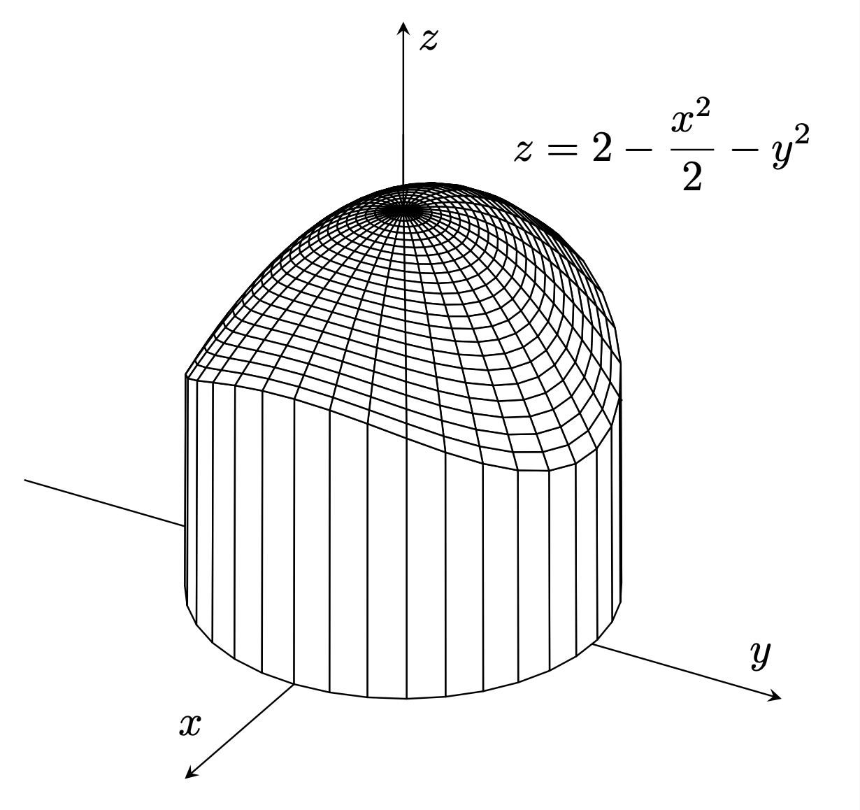
In general, `pgfplots` is a great tool for 3d plots. This is certainly the case if you plot a single surface, as in this example. If you have multiple intersecting plots, then you may have to work harder (but according to how I read the manual, the future may bring some tools that do such things automatically). To produces this plot, all we need to do is to use polar coordinates and a simple trick for the vertical wall: cut of the radius function via `rr(\x)=min(\x,1);`. Notice also that the axes are autmomatically almost right, but this is because they happen to be so in this example, so we only have to fix a stretch of the z-axis. In general, pgfplots does not compute the intersections of the axes with the surfaces, so we do have to do that ourselves. Note also that this plot does not really highlight some of the very nice features of `pgfplots` such as colorful shading with interpolated colors.
```
\documentclass[tikz,border=3mm]{standalone}
\usepackage{pgfplots}
\pgfplotsset{compat=1.17}
\begin{document}
\begin{tikzpicture}[line cap=round,line join=round,miter limit=5]
\begin{axis}[width=15cm,unit vector ratio=1 1 1,
view={120}{30},axis lines=center,
xtick=\empty,ytick=\empty,ztick=\empty,
xlabel={$x$},ylabel={$y$},zlabel={$z$},
xmin=-2,ymin=-2,zmin=0,
xmax=2,ymax=2,zmax=3,
declare function={f(\x,\y)=(\x<=1?2-\x*\x*(pow(cos(\y),2)/2+pow(sin(\y),2)):0);
rr(\x)=min(\x,1);}]
\addplot3[surf,fill=white,
colormap/blackwhite,point meta=0,
z buffer=sort,
samples y=36,
domain=0:1.04,y domain=0:360]
({rr(x)*cos(y)},{rr(x)*sin(y)},{f(x,y)});
\draw (0,0,2) -- (0,0,2.4);
\path (0,0.5,2.5) node[right]{$\displaystyle z=2-\frac{x^2}{2}-y^2$};
\end{axis}
\end{tikzpicture}
\end{document}
```
