I have a list of functions I define for multiple graphs along my course
```
%--------- Librairie de fonctions ---------
\tikzset{
declare function={
ZC(\x,\y)= pow(1+\x,-\y);
binom(\k,\n,\p)=\n!/(\k!*(\n-\k)!)*\p^\k*(1-\p)^(\n-\k);
Transfo(\a,\b,\c) = \a+\b+\c;
Spread(\a,\b,\c,\d,\e,\f)=\a*\d+\b*\e+\c*\f ;
normcdf(\x,\m,\SIG) = 1/(1 + exp(-0.07056*((\x-\m)/\SIG)^3 - 1.5976*(\x-\m)/\SIG));
invgauss(\a,\b) = sqrt(-2*ln(\a))*cos(deg(2*pi*\b));
d1(\x,\y,\KK,\RR,\SIG) = d2(\x,\y,\KK,\RR,\SIG) + (\SIG*(sqrt(\y)));
d2(\x,\y,\KK,\RR,\SIG) = (ln(\x/\KK)+(\RR-(pow(\SIG,2)/2)*\y))/(\SIG*(sqrt(\y)));
Nd1(\x,\y,\KK,\RR,\SIG) = normcdf(d1(\x,\y,\KK,\RR,\SIG),0,1);
Nd2(\x,\y,\KK,\RR,\SIG) = normcdf(d2(\x,\y,\KK,\RR,\SIG),0,1);
NPd1(\x,\y,\KK,\RR,\SIG) = Nprime(d1(\x,\y,\KK,\RR,\SIG));
NPd2(\x,\y,\KK,\RR,\SIG) = Nprime(d2(\x,\y,\KK,\RR,\SIG));
%... x100 more...
}
```
Since they're already written, why use `PythonTeX` (I thought about this interesting solution for calculations but a bazooka for a simple task) while I could use [mathematical-function-in-pgf-tikz](https://tex.stackexchange.com/questions/105766/using-mathematical-function-in-pgf-tikz) ?
However, I think the use of `\pgfmathparse{int(d1(\x,\y,\KK,\RR,\SIG)/100}\pgfmathresult` is quite heavy, so I must be doing someting wrong.
I could use a `\newcommand` like
```
\newcommand{\dOne}[5]{\pgfmathparse{int(d1(#1,#3,#2,#4,#5)*100)/100}\pgfmathresult}
```
but I lose the ability to name `\d1` my macro. I also believe what I do here is not elegant (d!mn French with elegance issues :))
Hence my question :
I'd like to have a fluid way of calling the functions and get the result (for a set of parameters) in my text.
```
MWE
\documentclass[tikz]{article}
%--------- Librairie de fonctions ---------
\tikzset{
declare function={
ZC(\x,\y)= pow(1+\x,-\y);
binom(\k,\n,\p)=\n!/(\k!*(\n-\k)!)*\p^\k*(1-\p)^(\n-\k);
Transfo(\a,\b,\c) = \a+\b+\c; %<- not pretty
Spread(\a,\b,\c,\d,\e,\f)=\a*\d+\b*\e+\c*\f ; %<-hum hum too
normcdf(\x,\m,\SIG) = 1/(1 + exp(-0.07056*((\x-\m)/\SIG)^3 - 1.5976*(\x-\m)/\SIG));
invgauss(\a,\b) = sqrt(-2*ln(\a))*cos(deg(2*pi*\b));
d1(\x,\y,\KK,\RR,\SIG) = d2(\x,\y,\KK,\RR,\SIG) + (\SIG*(sqrt(\y)));
d2(\x,\y,\KK,\RR,\SIG) = (ln(\x/\KK)+(\RR-(pow(\SIG,2)/2)*\y))/(\SIG*(sqrt(\y)));
Nd1(\x,\y,\KK,\RR,\SIG) = normcdf(d1(\x,\y,\KK,\RR,\SIG),0,1);
Nd2(\x,\y,\KK,\RR,\SIG) = normcdf(d2(\x,\y,\KK,\RR,\SIG),0,1);
NPd1(\x,\y,\KK,\RR,\SIG) = Nprime(d1(\x,\y,\KK,\RR,\SIG));
NPd2(\x,\y,\KK,\RR,\SIG) = Nprime(d2(\x,\y,\KK,\RR,\SIG));
%... x100 more...
}
\newcommand{\dOne}[5]{\pgfmathparse{int(d1(#1,#3,#2,#4,#5)*100)/100}\pgfmathresult}
\begin{document}
\dOne{100}{100}{1}{0}{0.25} result prints ok
\dOne{100}{100}{1}{0}{0.50} result prints ok
\dOne{100}{100}{1}{0}{0.75} result prints ok
\dOne{100}{100}{1}{0}{1.00} result prints ok
\end{document}
```
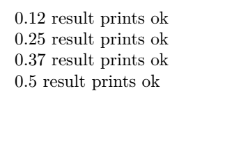
NB : I don't mention here the roundings of the results. I know it's a limitation.
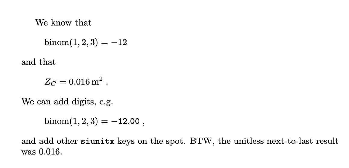
This is slight variation of [Rmano's nice answer](https://topanswers.xyz/tex?q=1557#a1809), merely for fun. I was wondering whether it is possible to steer the keys of `siunitx` with pgf keys. It is possible, but unless I am missing something basic one has to be a bit careful. (There are definitely improvements possible.) The command created here is `\Formula`, which takes one mandatory argument, the function that is to be parsed. And then there are options, which simultaneously allow one to steer `siunitx` stuff and pgf options. One can add `siunitx` keys with `si+={...}`. It does support things like `\Formula[si+={round-precision=4,math-rm=\mathtt}]{binom(1,2,3)}` which contain formatting macros like `\mathtt`. This works by copying the token mechanism of pgf keys. The parsed results also get remembered because sometimes one uses random numbers at some stage, and the subsequent results depend on the value of the random number. For instance, `StoredResult(2)` yields the result of the next-to-last computation. As usual, the rationale of using pgf keys here is to make the macro upgradable without losing backward compatibility.
```
\documentclass{article}
\usepackage[fleqn]{amsmath}% just for operatorname
\usepackage{tikz}
\usetikzlibrary{fpu}
\usepackage{siunitx}
\tikzset{
declare function={
ZC(\x,\y)= pow(1+\x,-\y);
binom(\k,\n,\p)=\n!/(\k!*(\n-\k)!)*\p^\k*(1-\p)^(\n-\k);
}}
\makeatletter
\newcounter{Formula@Stored@Results}
\pgfmathdeclarefunction*{StoredResult}{1}{%
\pgfmathifisint{#1}{\begingroup
\pgfkeys{/pgf/fpu,/pgf/fpu/output format=fixed}%
\pgfmathtruncatemacro{\pgfutil@tempi}{\number\value{Formula@Stored@Results}}%
\pgfmathtruncatemacro{\pgfutil@tempj}{\pgfutil@tempi-#1}%
\ifnum\pgfutil@tempj<1\relax
\typeout{Sorry, you wanted to retrieve the \pgfutil@tempi-#1th result, but only positive numbers are allowed.}
\edef\pgfmathresult{0}%
\else
\edef\pgfmathresult{\csname Formula@Stored@Results@\pgfutil@tempj\endcsname}%
\fi
\pgfmathsmuggle\pgfmathresult\endgroup}{\typeout{Sorry, StoredResult only accepts integer results.}}}
\newcommand{\Formula}[2][]{%
\begingroup
\stepcounter{Formula@Stored@Results}%
\pgfkeys{/pgf/fpu,/pgf/fpu/output format=fixed}%
\pgfkeys{/Formula/.cd,#1}%
\pgfkeysgetvalue{/Formula/sikeys}{\pgfutil@tempb}%
\pgfkeys@temptoks\expandafter\expandafter\expandafter{\csname pgfk@/Formula/sikeys\endcsname}%
\edef\pgfutil@tempa{\noexpand\sisetup{\the\pgfkeys@temptoks}}%
\pgfutil@tempa
\pgfmathparse{#2}%
\expandafter\xdef\csname Formula@Stored@Results@\number\value{Formula@Stored@Results}\endcsname{\pgfmathresult}%
\if@Formula@has@units
\SI{\pgfmathresult}{\@Formula@units}%
\else
\num{\pgfmathresult}%
\fi
\endgroup
}
\newif\if@Formula@has@units
\@Formula@has@unitsfalse
\pgfkeys{/Formula/.cd,has units/.is if=@Formula@has@units,
units/.code={\@Formula@has@unitstrue
\def\@Formula@units{#1}%
},sikeys/.initial={round-mode=figures,round-precision=2},
si+/.style={/Formula/sikeys/.append={,#1}}}
\makeatother
\begin{document}
We know that
\[\operatorname{binom}(1,2,3)=\Formula{binom(1,2,3)}\]
and that
\[Z_C= \Formula[units=\meter\squared]{ZC(3,3)}\;.\]
We can add digits, e.g.\
\[\operatorname{binom}(1,2,3)=\Formula[si+={round-precision=4,math-rm=\mathtt}]{binom(1,2,3)}\;,\]
and add other \texttt{siunitx} keys on the spot. BTW, the unitless next-to-last
result was \Formula{StoredResult(2)}.
\end{document}
```
I use the `declare function` a lot for my texts for students (especially exams, in order to easily create variants). The precision and range of the calculation is often a problem, so that I have to pre-scale units (forget about going with 46e-6 or things like that); having the same fuctionality in `l3fp` would be great). But alas, it's still very handy!

What I use normally is to get help by the `siunitx` package for formatting and printing. I have in my preamble:

```latex
\newcommand{\formula}[1]{%
    \pgfmathsetmacro{\rpval}{#1}%
    \num[round-mode=figures, round-precision=4]{\rpval}
}
\newcommand{\SIformula}[2]{%
    \pgfmathsetmacro{\rpval}{#1}%
    \SI[round-mode=figures, round-precision=4]{\rpval}{#2}%
}
```

and then in my text I can use

```latex
blah blah glub is \formula{binom(1,2,3)} and
quack \SIformula{ZC(3,3)}{\meter\squared} quack!
````

obviously you can pass additional parameters to control formats for printing, if needed. These macro are not expandable, but well --- they do work in most cases.
**I know this answer is not exactly what you are asking for but I think it is worth mentioning and might be useful to you or somebody else in one way or another.**
If the supreme WolframScript is more suitable for you than SageMath, then package [latexalpha2](https://ctan.org/pkg/latexalpha2?lang=en) is your new friend.
**However, it only works on Linux devices.** For Windows, I got you covered by having [this great answer](https://tex.stackexchange.com/a/579254/2288).
You must make sure first that you have first [Wolfram Engine](https://www.wolfram.com/engine/) and [WolframScript](https://www.wolfram.com/wolframscript/) are installed in this order.
Finally, run the command `wolframscript` once to activate your free account created when downloading WolframScript.
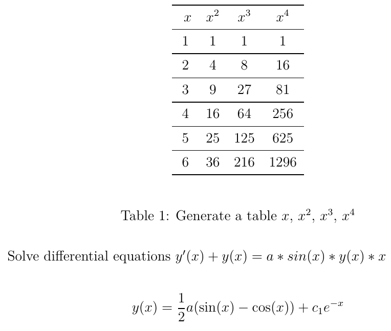
```
\documentclass[12pt,a4paper]{article}
% options: [local (default) or cloud] % [cache or nocache (default)]
% use the original package latexalpha2 for Linux
\usepackage{latexalpha2WinV2}
\parindent0pt
\begin{document}
\begin{figure}
\centering
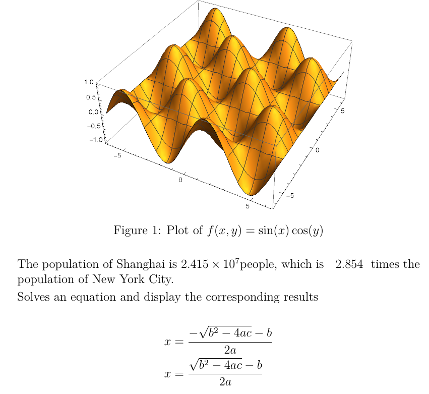
\wolframgraphics{Plot3D[Sin[x]Cos[y],{x,-2Pi,2Pi},{y,-2Pi,2Pi}]}{examplex}
\includegraphics{examplex.pdf}
\caption{Plot of $f(x,y)=\sin(x)\cos(y)$}
\end{figure}
The population of Shanghai is $\wolframalpha{Shanghai population}$, which
is \wolframalpha{ratio of Shanghai population and NYC population} times the
population of New York City.
\smallskip
Solves an equation and display the corresponding results
\wolframsolve{a x^2+b x+c==0}{x}
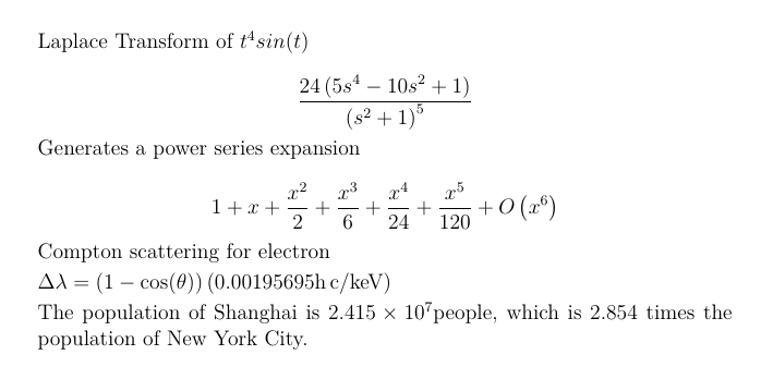
Laplace Transform of $t^4 sin(t)$
$$ \wolfram{LaplaceTransform[t^4 Sin[t],t,s]} $$
Generates a power series expansion
$$ \wolfram{Series[Exp[x],{x,0,5}]} $$
\smallskip
Compton scattering for electron \smallskip
$\wolframalpha{Compton scattering for electron}$
\begin{table}
\centering
\begin{tabular}{cccc} %set the correct number of columns!
\toprule
\wolframtable{Join[{{x,x^2,x^3,x^4}}, Table[{i,i^2,i^3,i^4},{i,6}]]}
\end{tabular}
\caption{Generate a table $x$, $x^2$, $x^3$, $x^4$}
\end{table}
\smallskip
The population of Shanghai is $\wolframalpha{Shanghai population}$, which is $\wolframalpha{ratio of Shanghai population and NYC population}$ times the
population of New York City.
\smallskip
Solve differential equations $y'(x) + y(x) = a *sin(x)*y(x)*x $
\wolframdsolve{y'[x]+y[x]==a Sin[x]}{y[x]}{x}
\end{document}
```
## Windows-tailored 'latexalpha2Win.sty'
```
%% This is file `latexalpha2Win.sty',
%% generated with the docstrip utility.
%%
%% The original source files were:
%%
%% latexalpha2.dtx (with options: `package')
%%
%% This is a generated file.
%%
%% Copyright (C) 2019 by Yi Liu <me@yliu.io>
%%
%% This file may be distributed and/or modified under the conditions of
%% the LaTeX Project Public License, either version 1.3c of this license
%% or (at your option) any later version. The latest version of this
%% license is in:
%%
%% http://www.latex-project.org/lppl.txt
%%
%% and version 1.3c or later is part of all distributions of LaTeX
%% version 2006/05/20 or later.
%%
%% modified for windows and luatex by Simon Dispa (2021)
%% https://tex.stackexchange.com/a/579254/2288
%%
%%%%%%%%%%%%%%%%%%%%%%%%%%%%%%%%%%%%%%%%%%%%%%%%%%%%%%%%%%%%%%%%%%%%%%%
\NeedsTeXFormat{LaTeX2e}
\ProvidesPackage{latexalpha2Win}[2021/01/18 v1.0 latexalpha2Win]
\RequirePackage{graphicx}
\RequirePackage{amsmath}
\RequirePackage{etoolbox}
\RequirePackage{pdftexcmds}
\RequirePackage{shellesc}
\RequirePackage{booktabs}
\newbool{ifcache}
\DeclareOption{local}{\def\la@platform{-local}}
\DeclareOption{cloud}{\def\la@platform{-cloud}}
\DeclareOption{cache}{\booltrue{ifcache}}
\DeclareOption{nocache}{\boolfalse{ifcache}}
\ExecuteOptions{nocache,local}
\ProcessOptions\relax
\begingroup
\makeatletter
\catcode`#=12
\catcode`&=12
\gdef\@hashchar{#}
\gdef\@ampchar{&}
\gdef\backslash{\@backslashchar}
\makeatother
\endgroup
\def\la@codetempfile{latexalpha2_code.tmp}
\def\la@resulttempfile{}
\def\la@currcodehash{}
\def\la@midrule{midrule}
\newcommand{\la@cleancodetempfile}{\immediate\write18{del /F /Q \la@codetempfile\space 2>NUL}}
\newcommand{\la@unknownoption}[2]{\PackageError{latexalpha2}{Unknown option '#2' for \@backslashchar #1}{}}
\newcommand{\la@executewolfram}[1]{%
% the optional command is the result output -format
\IfFileExists{\la@resulttempfile}{
\ifbool{ifcache}{}{\la@executewolframcore{#1}}
}{\la@executewolframcore{#1}}
}
\newcommand{\la@executewolframcore}[1]{%
% the optional command is the result output -format
\def\la@wolframscript{wolframscript -file \la@codetempfile\space -print -format #1 \la@platform\space> \la@resulttempfile}%
\immediate\write18{\la@wolframscript}%
}
\newcommand{\la@writecodefile}[2]{%
\gdef\la@currcodehash{\pdf@mdfivesum{#1#2}}%
\gdef\la@resulttempfile{#2_\la@currcodehash.out}%
\newwrite\tempfile%
\immediate\openout\tempfile=\la@codetempfile%
\immediate\write\tempfile{#1}%
\immediate\closeout\tempfile%
}
\def\la@texformat{tex}
\def\la@textformat{txt}
\def\la@wolframformat{wolfram}
\def\la@wolframtwoformat{wolfram2}
\def\la@pdfformat{pdf}
\def\la@pngformat{png}
\def\la@jpgformat{jpg}
\newcommand{\wolfram}[2][tex]{%
\def\la@currformat{#1}%
% write the temporary code file
\la@writecodefile{#2}{#1}%
% format the output result
\ifx \la@currformat \la@texformat \la@executewolfram{TeXForm} \else
\ifx \la@currformat \la@textformat \la@executewolfram{txt} \else
\ifx \la@currformat \la@wolframformat \la@executewolfram{} \else
\la@unknownoption{wolfram}{#1}
\fi\fi\fi
\input{\la@resulttempfile}%
\la@cleancodetempfile%
}
\newcommand{\wolframalpha}[2][tex]{%
\def\la@currformat{#1}%
% write the temporary code file
\la@writecodefile{WolframAlpha["#2","%
\ifx\la@currformat\la@textformat ShortAnswer\else
\ifx\la@currformat\la@wolframtwoformat Result\else
WolframResult\fi\fi
"]}{#1}%
% format the output result
\ifx \la@currformat \la@textformat \la@executewolfram{} \else
\ifx \la@currformat \la@wolframformat \la@executewolfram{} \else
\ifx \la@currformat \la@wolframtwoformat \la@executewolfram{} \else
\ifx \la@currformat \la@texformat \la@executewolfram{TeXForm} \else
\la@unknownoption{wolframalpha}{#1}
\fi\fi\fi\fi
\input{\la@resulttempfile}%
\la@cleancodetempfile%
}
\newcommand{\wolframgraphics}[3][pdf]{%
% write the temporary code file
\la@writecodefile{#2}{#1}%
% format the output result
\la@executewolfram{PDF}%
\immediate\write18{copy\space\la@resulttempfile\space#3.pdf >NUL}%
\la@cleancodetempfile%
}
\newcommand{\wolframsolve}[2]{%
% write the temporary code file
\la@writecodefile{"\@backslashchar\@backslashchar begin{flalign*}"<>StringJoin@@("\@ampchar"<>ToString[ToExpression["TeXForm"][#2]]<>"="<>ToString[ToExpression["TeXForm"][\@hashchar]]<>"\@backslashchar\@backslashchar\@backslashchar\@backslashchar"\@ampchar/@(#2/.Solve[#1, #2]))<>"\@backslashchar\@backslashchar end{flalign*}"}{}%
% format the output result
\la@executewolfram{txt}%
\input{\la@resulttempfile}%
\la@cleancodetempfile%
}
\newcommand{\wolframdsolve}[3]{%
% write the temporary code file
\la@writecodefile{"\@backslashchar\@backslashchar begin{flalign*}"<>StringJoin@@("\@ampchar"<>ToString[ToExpression["TeXForm"][#2]]<>"="<>ToString[ToExpression["TeXForm"][\@hashchar]]<>"\@backslashchar\@backslashchar\@backslashchar\@backslashchar"\@ampchar/@(#2/.DSolve[#1, #2, #3]))<>"\@backslashchar\@backslashchar end{flalign*}"}{}%
% format the output result
\la@executewolfram{txt}%
\input{\la@resulttempfile}%
\la@cleancodetempfile%
}
\newcommand{\wolframtable}[1]{%
\def\la@tablecode{StringJoin@@(%
(StringRiffle[("$"<>Slot[1]<>"$") \@ampchar/@ToString/@TeXForm/@(Slot[1]),"\space\@ampchar\space" ]
<> "\space\@backslashchar\@backslashchar\@backslashchar\@backslashchar\space\@backslashchar\@backslashchar\la@midrule\space")
\@ampchar/@(#1)
)}%
% write the temporary code file
\la@writecodefile{\la@tablecode}{tex}%
% format the output result
\la@executewolfram{Text}%
\la@cleancodetempfile%
\input{\la@resulttempfile}%
}
\AtBeginDocument{%
% Check if shell-escape is available
\ifcase\pdf@shellescape
\PackageError{latexalpha2}{Shell escape is not enabled, which is required to use latexalpha2}{}\or
\PackageInfo{latexalpha2}{Shell escape is successfully enabled}{}\or
\PackageError{latexalpha2}{Shell escape is not enabled, which is required to use latexalpha2}{}\fi
% Check if wolframscript is available
\immediate\write18{where wolframscript >latexalpha2_check.tmp 2>nul}%
% https://stackoverflow.com/a/35408403/2849383
%\immediate\write18{where /q wolframscript \ampchar echo \@percentchar ERRORLEVEL\@percentchar > latexalpha2_check.tmp}%
% https://superuser.com/a/1618520/452161
% https://superuser.com/a/718194/452161
% https://stackoverflow.com/a/25696405/2849383
\newread\wsreturncodefile%
\immediate\openin\wsreturncodefile=latexalpha2_check.tmp%
\readline\wsreturncodefile to \wsreturncode%
\immediate\closein\wsreturncodefile%
% https://tex.stackexchange.com/a/26873
\def\instring#1#2{TT\fi\begingroup\edef\x{\endgroup\noexpand\in@{#1}{#2}}\x\ifin@}%
\if\instring{{wolframscript.exe}}{\wsreturncode}
\PackageInfo{latexalpha2}{WolframScript is available}{}
\immediate\write18{del /F /Q latexalpha2_check.tmp 2>nul}\else
\immediate\write18{del /F /Q latexalpha2_check.tmp 2>nul}
\PackageError{latexalpha2}{WolframScript cannot be found, which is required to use latexalpha2}{}
\fi
}
\AtEndDocument{%
\ifbool{ifcache}{}{\immediate\write18{del /F /Q *.out 2>NUL} }
}
\endinput
%%
%% End of file `latexalpha2Win.sty'.
```If you don't mind externalization using a powerful computational engine, you might go with [SageMath](https://www.sagemath.org) using [sagetext](https://doc.sagemath.org/html/en/tutorial/sagetex.html).

```
% https://tex.stackexchange.com/a/578648/2288
\documentclass{article}
\usepackage{sagetex,siunitx,mathtools}
\parindent0pt
\begin{document}
\begin{sagesilent}
from sage.calculus.calculus import at
f(x) = exp(x)*sin(2*x)
out = r"%f"%(n(diff(f(x),x,2).subs(x=2)))
out1 = r"%4.2f"%(n(diff(f(x),x,2).subs(x=2)))
out2 = r"%f"%(n(diff(f(x),x,2).subs(x=2),digits=5))
dfx2 = r"\SI[round-mode=places, round-precision=3]{%f}{\kilo\metre}"%(n(diff(f(x),x,2).subs(x=2)))
\end{sagesilent}
The second derivative of $f$ is
\[
\frac{\mathrm{d}^{2}}{\mathrm{d}x^{2}} \sage{f(x)} =
\sage{diff(f, x, 2)(x)}.
\]
Here's a plot of $f$ from $-1$ to $1$:
\begin{center}
\sageplot[width=0.7\linewidth]{plot(f, -1, 1)}
\end{center}
Evaluating the derivatives at $x=2$ can be done in different ways
\begin{align}
&\frac{d}{dx}\sage{f(x)} = \sage{diff(f(x), x)}\\
&\sage{diff(f(x), x)} \text{ at } (x=1) \\
&= \sage{diff(f(x),x).subs(x=2)} = \sagestr{dfx2}\\
&\text{or}\\
&\sage{at(diff(f(x),x),x=2).n(digits=3)}
\end{align}
\sagestr{out}\\
\sagestr{out1}\\
\sagestr{out2}
\end{document}
```
---
# sagetex with arara
For automating the build process, you better use the following arara rule (if you are working on Windows) posted in this answer https://tex.stackexchange.com/a/596828/2288 after making `sagetex.sty` of SageMath [known to your latex distribution](https://doc.sagemath.org/html/en/tutorial/sagetex.html#sec-sagetex-install).
```
!config
# SageTeX-Rule for arara.
#
# Dear Windows-users, please check the paths
# pathToBashExecutive and pathToSageStartfile
# due to your Sage-installation!
#
identifier: sagetex
name: SageTeX
authors:
- TeXnician (Author)
- cis (Idea)
- Pedro J (final fix)
arguments: []
commands:
- name: A SageTeX Rule for arara
command: >
@{
pathToBashExecutive = "C:\\Program Files\\SageMath 9.1\\runtime\\bin\\bash";
pathToSageStartfile = "C:/Program Files/SageMath 9.1/runtime/opt/sagemath-9.1/sage";
pathOfCurrentWorkingFolder = currentFile().getParent();
theWindowsCommand = getCommand(pathToBashExecutive, "-l", pathToSageStartfile, "-c", "os.chdir(r'" + pathOfCurrentWorkingFolder + "'); load('" + getBasename(currentFile()) + ".sagetex.sage')");
return isWindows(theWindowsCommand, getCommand("sage", getBasename(reference) + ".sagetex.sage"));
}
```Thanks to the package of the day, I discovered the powerfull [numerica](https://ctan.org/pkg/numerica?lang=en)