**Question**

I need to automate calculations.

Strangely, declaring function by `\pgfmathdeclarefunction{PnL}` does not allow me to use the calculations when I call `Pnl{3.5}` and get the `y` coordinate.

Details in the code.

![TAGammaQuestion.png](/image?hash=4a19ce58f7f5a8b252088c61f05cdc9089547de50c82d4d3f744d57ec529fce0)

**Next step**

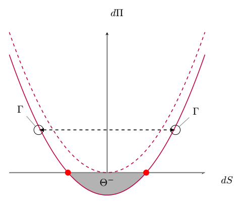
Of course animation :) The dashed curve will move along the y axis from its orinal position (dashed) to south, displaying more and more of the gray area.

```
\documentclass[border =2mm]{standalone}
\usepackage{tikz}
\usetikzlibrary{
	calc,
	intersections,
	positioning,
}
\usepackage{pgfplots}
\pgfplotsset{compat=1.16}

\usepgfplotslibrary{
	fillbetween,
}

\begin{document}

\newcommand*{\ShowIntersection}{
\fill 
    [name intersections={of=PnL and line, name=i, total=\t}] 
    [red, opacity=1, every node/.style={above left, black, opacity=1}] 
    \foreach \s in {1,...,\t}{(i-\s) circle (3pt)
        node [above] {}};
}

\begin{tikzpicture}
\pgfmathdeclarefunction{PnL}{0}{\pgfmathparse{0.5*(x^2)-2}}


\begin{axis}[%customaxis2,
   axis lines=middle,
   xtick={\empty},
   ytick={\empty},
   ytick       = {0},
   ticklabel style={font=\scriptsize},
   xlabel=$dS$,
   ylabel=$d\Pi$,
   xlabel style={at={(ticklabel* cs:1)}, xshift=12.5pt, anchor=north west},
   ylabel style={at={(ticklabel* cs:1)}, yshift=12.5pt, anchor=south west},
    samples     = 51,
%    domain      = -3:3,
%    xmin = -2, xmax = 5,
%    ymin = -5, ymax = 10,
  ]

% X axis
  \addplot[name path=line, gray, samples=2,no markers, line width=1pt] {0};
% curve
  \addplot[purple,dashed,samples=51,smooth,thick, mark=none, ] {PnL+2};
% dashed curve, inital position
  \addplot[purple,samples=51,smooth,name path=PnL, thick, mark=none, ] {PnL};

%filled area
  \addplot fill between[ 
    of = PnL and line, 
    split, % calculate segments
    every even segment/.style = {white}, %Only trick I found to avoi
    every odd segment/.style  = {gray!60}
  ] {};

% red intersection points to X axis
 \ShowIntersection  

% cord but too manual
  \coordinate (P) at (-3.5, 3.8);
%  \coordinate (P) at (-3.5, \Pnl(-3.5)  );
  \coordinate (Q) at (3.5, 3.8);

% too manual
\node[pin=130:$\Gamma$,draw=black,circle] at (-3.5, 3.8) {};
%\node[pin=130:$\Gamma$,draw=black,circle] at (-3.5, \Pnl(-3.5)) {};
\node[pin=40:$\Gamma$,draw=black,circle] at (3.5, 3.8) {};

% too manual
  \draw [latex-latex,dashed, thick, name path global=HorizontalLine] (P) -- (Q) node[above] {};

% too manual, but did not manage to place it in the center of the filled area
   \draw (0,-0.8) node {$\Theta^{-}$};	

\end{axis}
\end{tikzpicture}
\end{document}
```

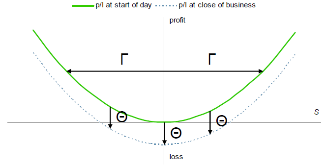
**Note**
The orginal graph
![Gammatheta.png](/image?hash=f50c7fc0d593143b57cdb199b1a05e3794152a5e99772690a4021fb6956e9c5c)