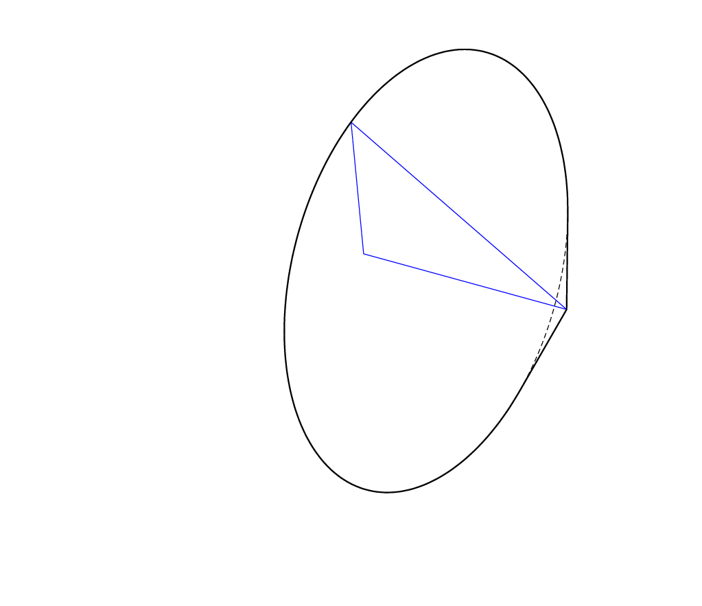
Here is some proof of principle for triangles. It computes the envelope of the rotation of a triangle around one of its edges. The critical angles are the same as [here](https://topanswers.xyz/tex?q=1218#a1447), only for a constant slope. I am not convinced that Ti*k*Z is made for such tasks, let alone for generalizations to arbitrary polygons. These codes require the newest version of [3dtools](https://github.com/marmotghost/tikz-3dtools) because I decided to add (a user interface to) the components of the normal to the library as they are getting used in various applications.
```
\documentclass[tikz,border=3mm]{standalone}
\usetikzlibrary{3dtools}% https://github.com/marmotghost/tikz-3dtools
\begin{document}
\foreach \AnglePhi in {5,15,...,355}
{\begin{tikzpicture}[line cap=butt,line join=round,
declare function={%
a=4.5;b=3;c=4;
tmpc(\u)=nscreenx*\u;%
sv1(\u)=-((-1*nscreenz*tmpc(\u)+sqrt(nscreeny*nscreeny+nscreenz*nscreenz-tmpc(\u)*tmpc(\u))*abs(nscreeny))%
/(nscreeny*nscreeny+nscreenz*nscreenz));%
sv2(\u)=(-(-1*nscreenz*tmpc(\u))+sqrt(nscreeny*nscreeny+nscreenz*nscreenz-tmpc(\u)*tmpc(\u))*abs(nscreeny))%
/(nscreeny*nscreeny+nscreenz*nscreenz);%
cv1(\u)=-((-1*nscreeny*tmpc(\u)+sqrt(nscreeny*nscreeny+nscreenz*nscreenz-tmpc(\u)*tmpc(\u))*abs(nscreenz))/(nscreeny*nscreeny+nscreenz*nscreenz));%
cv2(\u)=(-(-1*nscreeny*tmpc(\u))+sqrt(nscreeny*nscreeny+nscreenz*nscreenz-tmpc(\u)*tmpc(\u))*abs(nscreenz))/(nscreeny*nscreeny+nscreenz*nscreenz);%
tmpdisc(\u)=nscreeny*nscreeny+nscreenz*nscreenz-tmpc(\u)*tmpc(\u);%
}]
\path[use as bounding box] (-7,-6) rectangle (7,6) coordinate (TR);
%\path (6,-5) node[above left]{$\phi=\AnglePhi$};
\begin{scope}[3d/install view={phi=\AnglePhi,psi=0,theta=70}]
\path (a,0,0) coordinate (A) (0,b,0) coordinate (B) (0,0,c) coordinate (C)
[3d/define orthonormal dreibein];
\draw[blue] (A) -- (B) -- (C) -- cycle;
% height of the point (C) of the triangle
\pgfmathsetmacro{\myr}{TD("(C)-(A)o(ey)")}
% projection of (C) on line (A)--(B), i.e. distance from (A)
\pgfmathsetmacro{\myx}{TD("(C)-(A)o(ex)")}
\begin{scope}[x={(ex)},y={(ey)},z={(ez)},shift={(A)}]
\draw[thin,densely dashed,variable=\u,domain=0:360,samples=61,smooth cycle]
plot (\myx,{\myr*cos(\u)},{\myr*sin(\u)});
% slope of the first stretch
\pgfmathsetmacro{\myslope}{\myr/\myx}
\pgfmathtruncatemacro{\itest}{sign(tmpdisc(\myslope))}
\ifnum\itest>-1\relax
\pgfmathsetmacro{\angA}{Mod(720+atan2(sv1(\myslope),cv1(\myslope)),360)}
\pgfmathsetmacro{\angB}{Mod(720+atan2(sv2(\myslope),cv2(\myslope)),360)}
\pgfmathsetmacro{\angC}{min(\angA,\angB)}
\pgfmathsetmacro{\angD}{max(\angA,\angB)}
\pgfmathtruncatemacro{\jtest}{(screendepth(-1,0,0)>0)*((\angD-\angC)<180)}
\ifnum\jtest=1
\pgfmathsetmacro{\angC}{\angC+360}
\fi
\pgfmathtruncatemacro{\jtest}{(screendepth(-1,0,0)<0)*((\angD-\angC)>180)}
\ifnum\jtest=1
\pgfmathsetmacro{\angD}{\angD-360}
\fi
\draw[thick,variable=\u,domain=\angC:\angD,samples=61,smooth]
(A) -- plot (\myx,{\myr*cos(\u)},{\myr*sin(\u)}) -- cycle;
\else
\pgfmathtruncatemacro{\jtest}{sign(screendepth(-1,0,0))}
\ifnum\jtest=1
\draw[thick,variable=\u,domain=0:360,samples=61,smooth cycle]
plot (\myx,{\myr*cos(\u)},{\myr*sin(\u)});
\fi
\fi
\pgfmathsetmacro{\myL}{sqrt(a*a+b*b)-\myx}
\pgfmathsetmacro{\myslope}{-\myr/\myL}
\pgfmathtruncatemacro{\itest}{sign(tmpdisc(\myslope))}
\ifnum\itest>-1\relax
\pgfmathsetmacro{\angA}{Mod(720+atan2(sv1(\myslope),cv1(\myslope)),360)}
\pgfmathsetmacro{\angB}{Mod(720+atan2(sv2(\myslope),cv2(\myslope)),360)}
\pgfmathsetmacro{\angC}{min(\angA,\angB)}
\pgfmathsetmacro{\angD}{max(\angA,\angB)}
\pgfmathtruncatemacro{\jtest}{(screendepth(1,0,0)<0)*((\angD-\angC)<180)}
\ifnum\jtest<1
\pgfmathsetmacro{\angC}{\angC+360}
\fi
\pgfmathtruncatemacro{\jtest}{(screendepth(1,0,0)>0)*((\angD-\angC)>180)}
\ifnum\jtest=1
\pgfmathsetmacro{\angD}{\angD-360}
\fi
\draw[thick,variable=\u,domain=\angC:\angD,samples=61,smooth]
(B) -- plot (\myx,{\myr*cos(\u)},{\myr*sin(\u)}) -- cycle;
\else
\pgfmathtruncatemacro{\jtest}{sign(screendepth(1,0,0))}
\ifnum\jtest=1
\draw[thick,variable=\u,domain=0:360,samples=61,smooth cycle]
plot (\myx,{\myr*cos(\u)},{\myr*sin(\u)});
\fi
\fi
\end{scope}
\end{scope}
\end{tikzpicture}}
\end{document}
```
You can make it more solid-like by filling the contour.
```
\documentclass[tikz,border=3mm]{standalone}
\usetikzlibrary{3dtools}% https://github.com/marmotghost/tikz-3dtools
\begin{document}
\foreach \AnglePhi in {5,15,...,355}
{\begin{tikzpicture}[line cap=butt,line join=round,
declare function={%
a=4.5;b=3;c=4;
tmpc(\u)=nscreenx*\u;%
sv1(\u)=-((-1*nscreenz*tmpc(\u)+sqrt(nscreeny*nscreeny+nscreenz*nscreenz-tmpc(\u)*tmpc(\u))*abs(nscreeny))%
/(nscreeny*nscreeny+nscreenz*nscreenz));%
sv2(\u)=(-(-1*nscreenz*tmpc(\u))+sqrt(nscreeny*nscreeny+nscreenz*nscreenz-tmpc(\u)*tmpc(\u))*abs(nscreeny))%
/(nscreeny*nscreeny+nscreenz*nscreenz);%
cv1(\u)=-((-1*nscreeny*tmpc(\u)+sqrt(nscreeny*nscreeny+nscreenz*nscreenz-tmpc(\u)*tmpc(\u))*abs(nscreenz))/(nscreeny*nscreeny+nscreenz*nscreenz));%
cv2(\u)=(-(-1*nscreeny*tmpc(\u))+sqrt(nscreeny*nscreeny+nscreenz*nscreenz-tmpc(\u)*tmpc(\u))*abs(nscreenz))/(nscreeny*nscreeny+nscreenz*nscreenz);%
tmpdisc(\u)=nscreeny*nscreeny+nscreenz*nscreenz-tmpc(\u)*tmpc(\u);%
}]
\path[use as bounding box] (-7,-6) rectangle (7,6) coordinate (TR);
%\path (6,-5) node[above left]{$\phi=\AnglePhi$};
\begin{scope}[3d/install view={phi=\AnglePhi,psi=0,theta=70}]
\path (a,0,0) coordinate (A) (0,b,0) coordinate (B) (0,0,c) coordinate (C)
[3d/define orthonormal dreibein];
\draw[blue] (A) -- (B) -- (C) -- cycle;
% height of the point (C) of the triangle
\pgfmathsetmacro{\myr}{TD("(C)-(A)o(ey)")}
% projection of (C) on line (A)--(B), i.e. distance from (A)
\pgfmathsetmacro{\myx}{TD("(C)-(A)o(ex)")}
\begin{scope}[x={(ex)},y={(ey)},z={(ez)},shift={(A)}]
\draw[thin,densely dashed,variable=\u,domain=0:360,samples=61,smooth cycle]
plot (\myx,{\myr*cos(\u)},{\myr*sin(\u)});
% slope of the first stretch
\pgfmathsetmacro{\myslope}{\myr/\myx}
\pgfmathtruncatemacro{\itest}{sign(tmpdisc(\myslope))}
\ifnum\itest>-1\relax
\pgfmathsetmacro{\angA}{Mod(720+atan2(sv1(\myslope),cv1(\myslope)),360)}
\pgfmathsetmacro{\angB}{Mod(720+atan2(sv2(\myslope),cv2(\myslope)),360)}
\pgfmathsetmacro{\angC}{min(\angA,\angB)}
\pgfmathsetmacro{\angD}{max(\angA,\angB)}
\pgfmathtruncatemacro{\jtest}{(screendepth(-1,0,0)>0)*((\angD-\angC)<180)}
\ifnum\jtest=1
\pgfmathsetmacro{\angC}{\angC+360}
\fi
\pgfmathtruncatemacro{\jtest}{(screendepth(-1,0,0)<0)*((\angD-\angC)>180)}
\ifnum\jtest=1
\pgfmathsetmacro{\angD}{\angD-360}
\fi
\draw[thick,variable=\u,domain=\angC:\angD,samples=61,smooth,
fill=gray,fill opacity=0.5]
(A) -- plot (\myx,{\myr*cos(\u)},{\myr*sin(\u)}) -- cycle;
\else
\pgfmathtruncatemacro{\jtest}{sign(screendepth(-1,0,0))}
\ifnum\jtest=1
\draw[thick,variable=\u,domain=0:360,samples=61,smooth cycle,
fill=gray,fill opacity=0.5]
plot (\myx,{\myr*cos(\u)},{\myr*sin(\u)});
\fi
\fi
\pgfmathsetmacro{\myL}{sqrt(a*a+b*b)-\myx}
\pgfmathsetmacro{\myslope}{-\myr/\myL}
\pgfmathtruncatemacro{\itest}{sign(tmpdisc(\myslope))}
\ifnum\itest>-1\relax
\pgfmathsetmacro{\angA}{Mod(720+atan2(sv1(\myslope),cv1(\myslope)),360)}
\pgfmathsetmacro{\angB}{Mod(720+atan2(sv2(\myslope),cv2(\myslope)),360)}
\pgfmathsetmacro{\angC}{min(\angA,\angB)}
\pgfmathsetmacro{\angD}{max(\angA,\angB)}
\pgfmathtruncatemacro{\jtest}{(screendepth(1,0,0)<0)*((\angD-\angC)<180)}
\ifnum\jtest<1
\pgfmathsetmacro{\angC}{\angC+360}
\fi
\pgfmathtruncatemacro{\jtest}{(screendepth(1,0,0)>0)*((\angD-\angC)>180)}
\ifnum\jtest=1
\pgfmathsetmacro{\angD}{\angD-360}
\fi
\draw[thick,variable=\u,domain=\angC:\angD,samples=61,smooth,
fill=gray,fill opacity=0.5]
(B) -- plot (\myx,{\myr*cos(\u)},{\myr*sin(\u)}) -- cycle;
\else
\pgfmathtruncatemacro{\jtest}{sign(screendepth(1,0,0))}
\ifnum\jtest=1
\draw[thick,variable=\u,domain=0:360,samples=61,smooth cycle,
fill=gray,fill opacity=0.5]
plot (\myx,{\myr*cos(\u)},{\myr*sin(\u)});
\fi
\fi
\end{scope}
\end{scope}
\end{tikzpicture}}
\end{document}
```
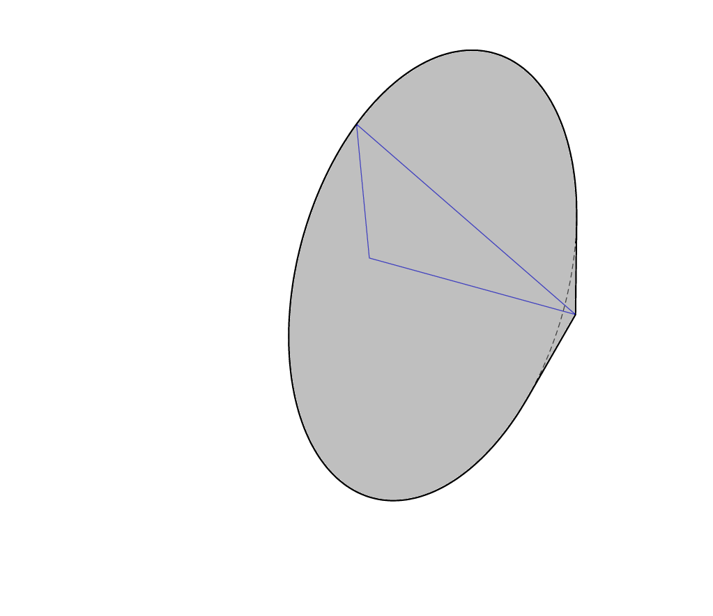
Unfortunately I do not know of a good way to add realistic shading.