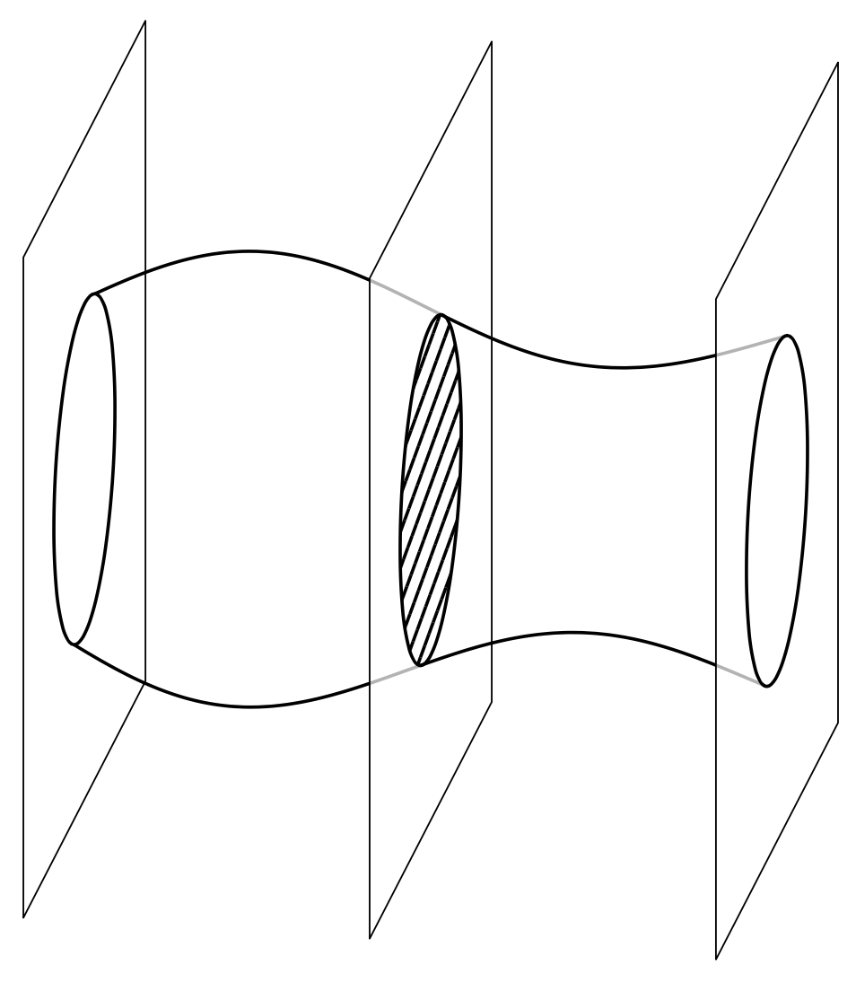
This answer comes in three parts, sorted by increasing complexity. The IMHO "best" solution is at the end. Let us start with a very simpleminded proposal, which only works in the limit of small phi, i.e. the second argument of `\tdplotsetmaincoords{<theta>}{<phi>}` needs to be such that the absolute value of its sine is small. Next, a function `R` is introduced that specifies the radius of the volume as a function of `x`. Then the planes and volume are drawn step by step.
```
\documentclass[border=2mm,12pt,tikz]{standalone}
\usepackage{tikz-3dplot}
\usetikzlibrary{patterns.meta}
\begin{document}
\tdplotsetmaincoords{70}{10}
\begin{tikzpicture}[tdplot_main_coords,scale=1,
line cap=butt,line join=round,
declare function={R(\u)=1.5+sin(\u*60)/(2+\u/6);}]
\tikzset{icircle/.style={thick},iplane/.style={fill=white,fill opacity=0.7},
stretch/.style={thick,domain=#1,insert path={%
plot[smooth,variable=\u]
(\u,{R(\u)*cos(\tdplotmaintheta)},{R(\u)*sin(\tdplotmaintheta)})
plot[smooth,variable=\u]
(\u,{R(\u)*cos(\tdplotmaintheta+180)},{R(\u)*sin(\tdplotmaintheta+180)})
}}}
\newcommand\DrawIntersectingPlane[2][]{%
\begin{scope}[canvas is yz plane at x=#2,transform shape,#1]
\draw[iplane] (3,3) -- (-3,3) -- (-3,-3)-- (3,-3) -- cycle;
\draw[icircle] (0,0) circle[radius={R(#2)}];
\end{scope}}
\DrawIntersectingPlane{0}
\draw[stretch=0:3];
\DrawIntersectingPlane[icircle/.append style={pattern={Lines[angle=70,distance={3pt}]}}]{3}
\draw[stretch=3:6];
\DrawIntersectingPlane{6}
\end{tikzpicture}
\end{document}
```
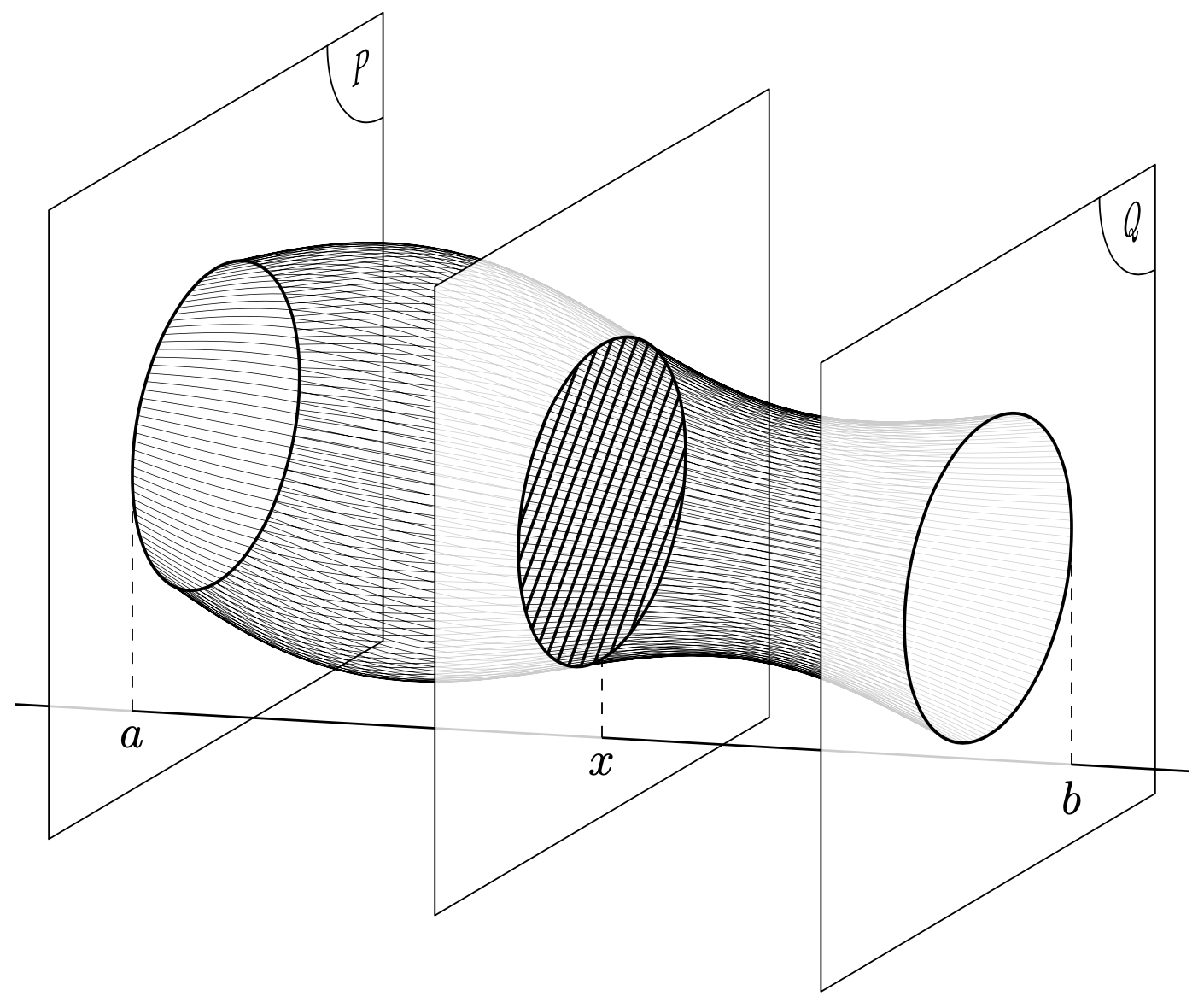
Once you want to add annotations on the planes, things become more complicated as you probably want to change the view angle, and the simpleminded solution ceases to be sufficiently accurate. As shown below, the contour of the volume can be computed analytically. Before doing that, let us just add 120 plots at the surface to give a 3d impression. Obviously, one may consider using `pgfplots`, but here is just another rather simpleminded approach.
```
\documentclass[border=2mm,12pt,tikz]{standalone}
\usepackage{tikz-3dplot}
\usetikzlibrary{intersections,patterns.meta}
\begin{document}
\tdplotsetmaincoords{70}{30}
\begin{tikzpicture}[tdplot_main_coords,scale=1,
line cap=butt,line join=round,
declare function={R(\u)=1.5+sin(\u*45)/(2+\u/8);},
icircle/.style={thick},
iplane/.style={fill=white,fill opacity=0.8},
iline/.style={semithick},
extra/.code={},annot/.code={\tikzset{extra/.code={#1}}}]
\newcommand\DrawIntersectingPlane[2][]{%
\begin{scope}[canvas is yz plane at x=#2,transform shape,#1]
\draw[iplane] (3,3) -- (-3,3) -- (-3,-3)-- (3,-3) -- cycle;
\draw[icircle] (0,0) circle[radius={R(#2)}];
\tikzset{extra}
\end{scope}}
\newcommand\DrawStretch[2][]{%
\draw[ultra thin,domain=#2,#1] foreach \Ang in {0,3,...,357}
{
plot[smooth,variable=\u]
(\u,{R(\u)*cos(\Ang)},{R(\u)*sin(\Ang)})};
}
\draw[iline] (-1,{-1.5*5/4},-2.25) -- (0,{-1.5},-2.25);
\DrawIntersectingPlane[annot={%
\path (2.9,2.9) node[below left,transform shape]{$P$};
\draw (2,3) arc[start angle=180,end angle=270,radius=1];
\draw[dashed] (-1.5,-2.25) node[below,transform shape=false]{$a$} -- (-1.5,0);
}]{0}
\draw[iline] (0,{-1.5},-2.25) -- (4,0,-2.25);
\DrawStretch{0:4}
\DrawIntersectingPlane[icircle/.append style={pattern={Lines[angle=70,distance={3pt}]}},
annot={%
\draw[dashed] (0,-2.25) node[below,transform shape=false]{$x$} -- (0,-1.5);
}]{4}
\draw[iline] (4,0,-2.25) -- (8,1.5,-2.25);
\DrawStretch{4:8}
\DrawIntersectingPlane[annot={%
\path (2.9,2.9) node[below left,transform shape]{$Q$};
\draw (2,3) arc[start angle=180,end angle=270,radius=1];
\draw[dashed] (1.5,-2.25) node[below,transform shape=false]{$b$} -- (1.5,0);
}]{8}
\draw[iline] (8,1.5,-2.25) -- (9,{1.5*5/4},-2.25) ;
\end{tikzpicture}
\end{document}
```
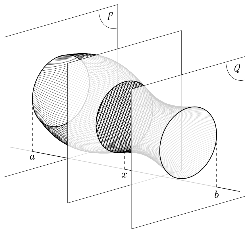
If you change the view angles to `\tdplotsetmaincoords{70}{50}`, you get
The contour can be computed analytically.
leading to
And here is the LaTeX code for this derivation and result.
```
\documentclass[fleqn]{article}
\usepackage{geometry}
\usepackage{amsmath}
\usepackage{tikz}
\usepackage{tikz-3dplot}
\usetikzlibrary{patterns.meta}
\begin{document}
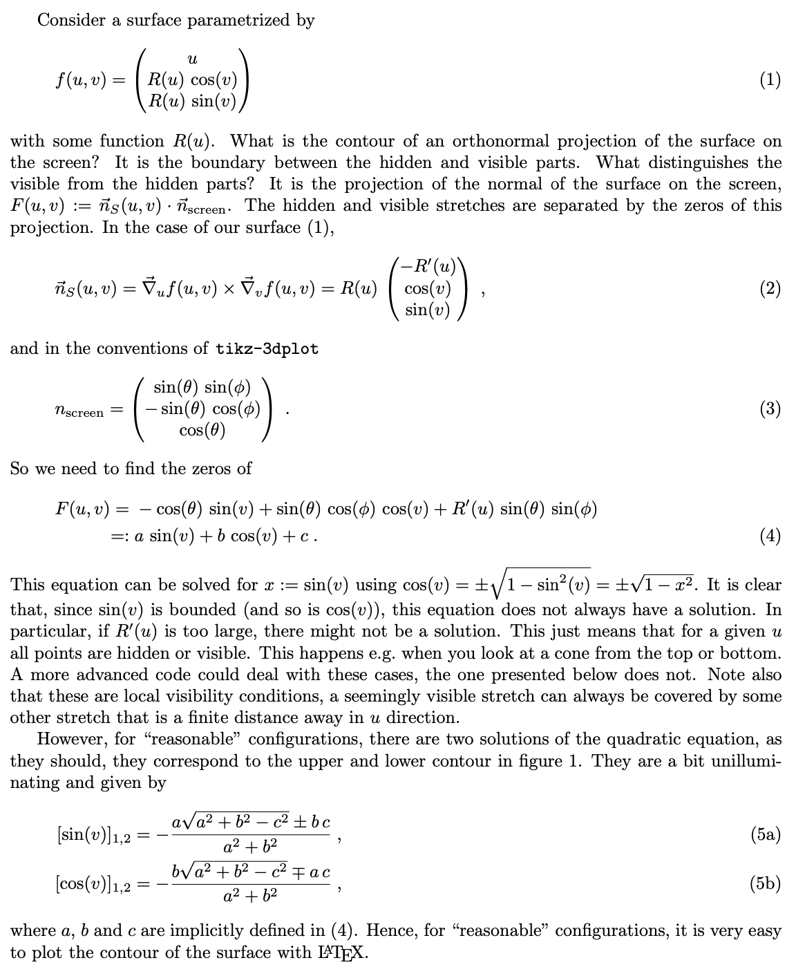
Consider a surface parametrized by
\begin{equation}\label{eq:f}
f(u,v)=\begin{pmatrix}
u\\ R(u)\,\cos (v)\\ R(u)\,\sin (v)
\end{pmatrix}
\end{equation}
with some function $R(u)$. What is the contour of an orthonormal projection of the
surface on the screen? It is the boundary between the hidden and visible parts.
What distinguishes the visible from the hidden parts? It is the projection of
the normal of the surface on the screen, $F(u,v):=\vec n_S(u,v)\cdot \vec
n_\mathrm{screen}$. The hidden and visible stretches are separated by the zeros
of this projection. In the case of our surface \eqref{eq:f},
\begin{equation}
\vec n_S(u,v)=\vec\nabla_u f(u,v)\times \vec\nabla_v f(u,v)
=R(u)\,\begin{pmatrix}
-R'(u)\\ \cos (v)\\ \sin (v)
\end{pmatrix}\;,
\end{equation}
and in the conventions of \texttt{tikz-3dplot}
\begin{equation}
n_\mathrm{screen}=\begin{pmatrix}
\sin(\theta)\,\sin (\phi)\\
-\sin (\theta )\,\cos(\phi)\\
\cos (\theta)
\end{pmatrix}\;.
\end{equation}
So we need to find the zeros of
\begin{align}
F(u,v)={}&{}-\cos (\theta)\,\sin (v)+
\sin (\theta )\,\cos(\phi)\,\cos (v)+ R'(u)\,\sin(\theta)\,\sin (\phi)\notag\\
=:{}&{}a\,\sin (v)+b\,\cos(v)+c\;.\label{eq:vcrit}
\end{align}
This equation can be solved for $x:=\sin (v)$ using
$\cos(v)=\pm\sqrt{1-\sin^2(v)}=\pm\sqrt{1-x^2}$. It is clear that, since $\sin
(v)$ is bounded (and so is $\cos(v)$), this equation does not always have a
solution. In particular, if $R'(u)$ is too large, there might not be a solution.
This just means that for a given $u$ all points are hidden or visible. This
happens e.g.\ when you look at a cone from the top or bottom. A more advanced
code could deal with these cases, the one presented below does not. Note also
that these are local visibility conditions, a seemingly visible stretch can
always be covered by some other stretch that is a finite distance away in $u$
direction.
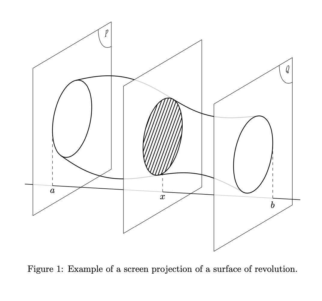
However, for ``reasonable'' configurations, there are two solutions of the
quadratic equation, as they should, they correspond to the upper and lower
contour in figure~\ref{fig:example}. They are a bit unilluminating and given by
\begin{subequations}\label{eq:cvandsv}
\begin{align}
[\sin(v)]_{1,2}&=-\frac{a \sqrt{a^2+b^2-c^2}\pm b\,c}{a^2+b^2}\;,\\
[\cos(v)]_{1,2}&=-\frac{b \sqrt{a^2+b^2-c^2}\mp a\,c}{a^2+b^2}\;,
\end{align}
\end{subequations}
where $a$, $b$ and $c$ are implicitly defined in \eqref{eq:vcrit}. Hence, for
``reasonable'' configurations, it is very easy to plot the contour of the
surface with \LaTeX.
\begin{figure}[h]
\centering
\tdplotsetmaincoords{70}{30}%
\begin{tikzpicture}[tdplot_main_coords,scale=1,
line cap=butt,line join=round,%trig format=rad,
declare function={%
R(\u)=1.5+sin(\u*45)/(2+\u/8);%<- input
Rprime(\u)=(R(\u+0.01)-R(\u-0.01))/0.02;%<- numerical derivative
a=cos(\tdplotmainphi)*sin(\tdplotmaintheta);% see equation {eq:vcrit}
b=-1*cos(\tdplotmaintheta);%
c(\u)=sin(\tdplotmaintheta)*sin(\tdplotmainphi)*Rprime(\u);%
sv1(\u)=-((b*c(\u)+sqrt(a*a+b*b-c(\u)*c(\u))*abs(a))/(a*a+b*b));% see equation {eq:cvandsv}
sv2(\u)=(-(b*c(\u))+sqrt(a*a+b*b-c(\u)*c(\u))*abs(a))/(a*a+b*b);%
cv1(\u)=-((a*c(\u)+sqrt(a*a+b*b-c(\u)*c(\u))*abs(b))/(a*a+b*b));%
cv2(\u)=(-(a*c(\u))+sqrt(a*a+b*b-c(\u)*c(\u))*abs(b))/(a*a+b*b);%
},
icircle/.style={thick},
iplane/.style={fill=white,fill opacity=0.8},
iline/.style={semithick},
extra/.code={},annot/.code={\tikzset{extra/.code={#1}}}]
\newcommand\DrawIntersectingPlane[2][]{%
\begin{scope}[canvas is yz plane at x=#2,transform shape,#1]
\draw[iplane] (3,3) -- (-3,3) -- (-3,-3)-- (3,-3) -- cycle;
\draw[icircle] (0,0) circle[radius={R(#2)}];
\tikzset{extra}
\end{scope}}
%
\draw[iline] (-1,{-1.5*5/4},-2.25) -- (0,{-1.5},-2.25);
\DrawIntersectingPlane[annot={%
\path (2.9,2.9) node[below left,transform shape]{$P$};
\draw (2,3) arc[start angle=180,end angle=270,radius=1];
\draw[dashed] (-1.5,-2.25) node[below,transform shape=false]{$a$} -- (-1.5,0);
}]{0}
\draw[iline] (0,{-1.5},-2.25) -- (4,0,-2.25);
\draw[thick,smooth,variable=\u,domain=0:4]
plot (\u,{R(\u)*cv1(\u)},{R(\u)*sv1(\u)})
plot (\u,{R(\u)*cv2(\u)},{R(\u)*sv2(\u)});
\DrawIntersectingPlane[icircle/.append style={pattern={Lines[angle=70,distance={3pt}]}},
annot={%
\draw[dashed] (0,-2.25) node[below,transform shape=false]{$x$} -- (0,-1.5);
}]{4}
\draw[iline] (4,0,-2.25) -- (8,1.5,-2.25);
\draw[thick,smooth,variable=\u,domain=4:8]
plot (\u,{R(\u)*cv1(\u)},{R(\u)*sv1(\u)})
plot (\u,{R(\u)*cv2(\u)},{R(\u)*sv2(\u)});
;
\DrawIntersectingPlane[annot={%
\path (2.9,2.9) node[below left,transform shape]{$Q$};
\draw (2,3) arc[start angle=180,end angle=270,radius=1];
\draw[dashed] (1.5,-2.25) node[below,transform shape=false]{$b$} -- (1.5,0);
}]{8}
\draw[iline] (8,1.5,-2.25) -- (9,{1.5*5/4},-2.25) ;
\end{tikzpicture}
\caption{Example of a screen projection of a surface of revolution.}
\label{fig:example}
\end{figure}
\end{document}
```
Please note that, when computing the derivative of `R(u)`, you need to remember the weird convention of pgf to use degrees (by default). Needless to say that the analogous analytical formulae can be used for other tools such as pgfplots. When doing so, one has to check the conventions for theta and phi, unfortunately. Hoewever, as one can see one really only needs the normal on the screen.
This is now a sufficiently fast code that can be animated. In this animation, a numerical derivative is employed, which seems to do the job, at least in this case. So all you need to specify is `R(\u)`.
```
\documentclass[border=2mm,12pt,tikz]{standalone}
\usepackage{tikz-3dplot}
\usetikzlibrary{patterns.meta}
\begin{document}
\foreach \AnglePhi in {10,15,...,50,45,40,...,15}
{\tdplotsetmaincoords{70}{\AnglePhi}
\begin{tikzpicture}[tdplot_main_coords,scale=1,
line cap=butt,line join=round,%trig format=rad,
declare function={%
R(\u)=1.5+sin(\u*45)/(2+\u/8);%
Rprime(\u)=(R(\u+0.01)-R(\u-0.01))/0.02;%
a=cos(\tdplotmainphi)*sin(\tdplotmaintheta);%
b=-1*cos(\tdplotmaintheta);%
c(\u)=sin(\tdplotmaintheta)*sin(\tdplotmainphi)*Rprime(\u);%
sv1(\u)=-((b*c(\u) + sqrt(a*a + b*b -
c(\u)*c(\u))*abs(a))/(a*a + b*b));
sv2(\u)=(-(b*c(\u)) + sqrt(a*a + b*b -
c(\u)*c(\u))*abs(a))/(a*a + b*b);
cv1(\u)=-((a*c(\u) + sqrt(a*a + b*b -
c(\u)*c(\u))*abs(b))/(a*a + b*b));
cv2(\u)=(-(a*c(\u)) + sqrt(a*a + b*b -
c(\u)*c(\u))*abs(b))/(a*a + b*b);
},
icircle/.style={thick},
iplane/.style={fill=white,fill opacity=0.8},
iline/.style={semithick},
extra/.code={},annot/.code={\tikzset{extra/.code={##1}}}]
\path[tdplot_screen_coords,use as bounding box] (-3,-7) rectangle (10,5);
\newcommand\DrawIntersectingPlane[2][]{%
\begin{scope}[canvas is yz plane at x=##2,transform shape,##1]
\draw[iplane] (3,3) -- (-3,3) -- (-3,-3)-- (3,-3) -- cycle;
\draw[icircle] (0,0) circle[radius={R(##2)}];
\tikzset{extra}
\end{scope}}
%
\draw[iline] (-1,{-1.5*5/4},-2.25) -- (0,{-1.5},-2.25);
\DrawIntersectingPlane[annot={%
\path (2.9,2.9) node[below left,transform shape]{$P$};
\draw (2,3) arc[start angle=180,end angle=270,radius=1];
\draw[dashed] (-1.5,-2.25) node[below,transform shape=false]{$a$} -- (-1.5,0);
}]{0}
\draw[iline] (0,{-1.5},-2.25) -- (4,0,-2.25);
\draw[thick,smooth,variable=\u,domain=0:4]
plot (\u,{R(\u)*cv1(\u)},{R(\u)*sv1(\u)})
plot (\u,{R(\u)*cv2(\u)},{R(\u)*sv2(\u)});
\DrawIntersectingPlane[icircle/.append style={pattern={Lines[angle=70,distance={3pt}]}},
annot={%
\draw[dashed] (0,-2.25) node[below,transform shape=false]{$x$} -- (0,-1.5);
}]{4}
\draw[iline] (4,0,-2.25) -- (8,1.5,-2.25);
\draw[thick,smooth,variable=\u,domain=4:8]
plot (\u,{R(\u)*cv1(\u)},{R(\u)*sv1(\u)})
plot (\u,{R(\u)*cv2(\u)},{R(\u)*sv2(\u)});
;
\DrawIntersectingPlane[annot={%
\path (2.9,2.9) node[below left,transform shape]{$Q$};
\draw (2,3) arc[start angle=180,end angle=270,radius=1];
\draw[dashed] (1.5,-2.25) node[below,transform shape=false]{$b$} -- (1.5,0);
}]{8}
\draw[iline] (8,1.5,-2.25) -- (9,{1.5*5/4},-2.25) ;
\end{tikzpicture}}
\end{document}
```
Of course, you can also animate the `x` position to provide an intuition for the volume integration.
```
\documentclass[border=2mm,12pt,tikz]{standalone}
\usepackage{tikz-3dplot}
\usetikzlibrary{patterns.meta}
\begin{document}
\foreach \xpos in {0.4,0.8,...,7.6}
{\tdplotsetmaincoords{70}{40}
\begin{tikzpicture}[tdplot_main_coords,scale=1,
line cap=butt,line join=round,%trig format=rad,
declare function={%
R(\u)=1.5+sin(\u*45)/(2+\u/8);%
Rprime(\u)=(R(\u+0.01)-R(\u-0.01))/0.02;%
a=cos(\tdplotmainphi)*sin(\tdplotmaintheta);%
b=-1*cos(\tdplotmaintheta);%
c(\u)=sin(\tdplotmaintheta)*sin(\tdplotmainphi)*Rprime(\u);%
sv1(\u)=-((b*c(\u) + sqrt(a*a + b*b -
c(\u)*c(\u))*abs(a))/(a*a + b*b));
sv2(\u)=(-(b*c(\u)) + sqrt(a*a + b*b -
c(\u)*c(\u))*abs(a))/(a*a + b*b);
cv1(\u)=-((a*c(\u) + sqrt(a*a + b*b -
c(\u)*c(\u))*abs(b))/(a*a + b*b));
cv2(\u)=(-(a*c(\u)) + sqrt(a*a + b*b -
c(\u)*c(\u))*abs(b))/(a*a + b*b);
},
icircle/.style={thick},
iplane/.style={fill=white,fill opacity=0.8},
iline/.style={semithick},
extra/.code={},annot/.code={\tikzset{extra/.code={##1}}}]
\path[tdplot_screen_coords,use as bounding box] (-3,-7) rectangle (10,5);
\newcommand\DrawIntersectingPlane[2][]{%
\begin{scope}[canvas is yz plane at x=##2,transform shape,##1]
\draw[iplane] (3,3) -- (-3,3) -- (-3,-3)-- (3,-3) -- cycle;
\draw[icircle] (0,0) circle[radius={R(##2)}];
\tikzset{extra}
\end{scope}}
%
\DrawIntersectingPlane[annot={%
\path (2.9,2.9) node[below left,transform shape]{$P$};
\draw (2,3) arc[start angle=180,end angle=270,radius=1];
\draw[dashed] (0,-2.25) node[below,transform shape=false]{$a$} -- (0,{-R(0)});
}]{0}
\draw[iline] (0,0,-2.25) -- (\xpos,0,-2.25);
\draw[thick,smooth,variable=\u,domain=0:\xpos]
plot (\u,{R(\u)*cv1(\u)},{R(\u)*sv1(\u)})
plot (\u,{R(\u)*cv2(\u)},{R(\u)*sv2(\u)});
\DrawIntersectingPlane[icircle/.append style={pattern={Lines[angle=70,distance={3pt}]}},
annot={%
\draw[dashed] (0,-2.25) node[below,transform shape=false]{$x$} -- (0,{-R(\xpos)});
}]{\xpos}
\draw[iline] (\xpos,0,-2.25) -- (8,0,-2.25);
\draw[thick,smooth,variable=\u,domain=\xpos:8]
plot (\u,{R(\u)*cv1(\u)},{R(\u)*sv1(\u)})
plot (\u,{R(\u)*cv2(\u)},{R(\u)*sv2(\u)});
\DrawIntersectingPlane[annot={%
\path (2.9,2.9) node[below left,transform shape]{$Q$};
\draw (2,3) arc[start angle=180,end angle=270,radius=1];
\draw[dashed] (0,-2.25) node[below,transform shape=false]{$b$} -- (0,{-R(8)});
}]{8}
\end{tikzpicture}}
\end{document}
```