i-one

I was experimenting in preparation for the other post and noticed how query optimizer makes a choice between trivial and full cost-based optimization for the same query sometimes. Observed behavior was something that I was not aware of and not able to find mentioned, that made me curious to dig into it. Let's proceed with an example.
## **Setup**
The following table
```sql
CREATE TABLE [#Data]
(
[K] int IDENTITY(1,1) NOT NULL PRIMARY KEY CLUSTERED,
[A] int NOT NULL,
[B] tinyint NULL,
[C] varchar(20) NOT NULL
);
GO
CREATE INDEX [IX_Data_B] ON [#Data] ([B]) INCLUDE ([C]);
GO
```
along with some data
```sql
INSERT INTO [#Data] WITH (TABLOCK) ([A], [B], [C])
SELECT TOP (1000)
1,
NULL,
REPLICATE('C', IIF(ROW_NUMBER() OVER (ORDER BY @@SPID) / 963 = 0, 10, 20))
FROM sys.all_columns;
```
will serve purpose of the demonstration.
## **The Query**
Now that we have table and data, imagine that we also have some very simple `SELECT` query with `WHERE` predicate, like
```sql
SELECT [K]
FROM [#Data]
WHERE [A] = 2;
```
There is no suitable non-clustered index on the `#Data` table to support this query, and so its execution plan is the plain Clustered Index Scan
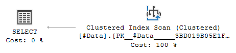
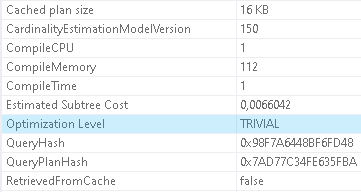
Properties of the execution plan indicate that it has resulted from trivial optimization
Now let's insert a row to the `#Data` table
```sql
INSERT INTO [#Data] ([A], [B], [C])
VALUES (1, NULL, 'C');
```
and obtain execution plan of the query again
```sql
SELECT [K]
FROM [#Data]
WHERE [A] = 2
OPTION (RECOMPILE);
```
(option `RECOMPILE` is added to ensure that cached plan is not reused). Graphical representation of the execution plan is just the same, so I will not repeat it. This time, however, the execution plan has resulted from full cost-based optimization
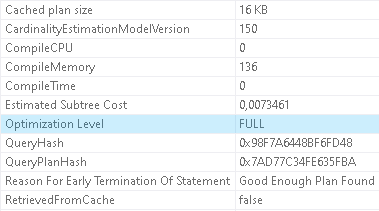
Why has the optimization level changed?
Okay, what are the things that can prevent trivial optimization in this case?
- Subqueries, joins, inequality predicates[^1]? No, not applicable.
- Estimated cost compared to cost threshold for parallelism? No, query cost is far below CTFP (which is set to its default value of 5 units).
What else?
- Non-covering index presence[^2][^3]? Hmm... it's interesting, as there is the non-clustered index `IX_Data_B`, which is non-covering for the subject query.
It seems that there is more than just presence though, because of non-covering index was there since the beginning, and optimization level has changed after _data change_. There must be something else, some additional factor.
Now let's change fill-factor of the non-covering index as follows
```sql
ALTER INDEX [IX_Data_B] ON [#Data] REBUILD WITH (FILLFACTOR = 75);
```
and obtain execution plan once again. Properties of the execution plan indicate that optimization level has reverted to trivial
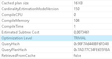
This gives one the strong hint as to what the additional factor is.
## **Storage Statistics Do Matter**
I must confess that "some data" that was used in the Setup section is carefully prepared data actually.
Following are the storage statistics returned by `sys.dm_db_index_physical_stats` data management function for the `#Data` table. At initial population, amount of space taken by the non-clustered index was the same as that of the clustered index
| index_id | index_name | index_type_desc | index_depth | index_level | page_count | record_count |
| --------:| ---------- | --------------- | -----------:| -----------:| ----------:| ------------:|
| 1 | PK_#Data_3BD019B05E1F9831 | CLUSTERED INDEX | 2 | 0 | 4 | 1000 |
| 1 | PK_#Data_3BD019B05E1F9831 | CLUSTERED INDEX | 2 | 1 | 1 | 4 |
| 2 | IX_Data_B | NONCLUSTERED INDEX | 2 | 0 | 4 | 1000 |
| 2 | IX_Data_B | NONCLUSTERED INDEX | 2 | 1 | 1 | 4 |
Insertion of just one row caused growth of the leaf level of clustered index
| index_id | index_name | index_type_desc | index_depth | index_level | page_count | record_count |
| --------:| ---------- | --------------- | -----------:| -----------:| ----------:| ------------:|
| 1 | PK_#Data_3BD019B05E1F9831 | CLUSTERED INDEX | 2 | 0 | 5 | 1001 |
| 1 | PK_#Data_3BD019B05E1F9831 | CLUSTERED INDEX | 2 | 1 | 1 | 5 |
| 2 | IX_Data_B | NONCLUSTERED INDEX | 2 | 0 | 4 | 1001 |
| 2 | IX_Data_B | NONCLUSTERED INDEX | 2 | 1 | 1 | 4 |
and rebuild of the non-clustered index reinstated parity again
| index_id | index_name | index_type_desc | index_depth | index_level | page_count | record_count |
| --------:| ---------- | --------------- | -----------:| -----------:| ----------:| ------------:|
| 1 | PK_#Data_3BD019B05E1F9831 | CLUSTERED INDEX | 2 | 0 | 5 | 1001 |
| 1 | PK_#Data_3BD019B05E1F9831 | CLUSTERED INDEX | 2 | 1 | 1 | 5 |
| 2 | IX_Data_B | NONCLUSTERED INDEX | 2 | 0 | 5 | 1001 |
| 2 | IX_Data_B | NONCLUSTERED INDEX | 2 | 1 | 1 | 5 |
During the optimization, storage statistics of the table itself (clustered index or heap) and available indexes are checked. Trivial optimization for the subject query is possible, if number of leaf-level pages for the `IX_Data_B` index equals to or grater than that of the clustered index. This is necessary condition. Speaking more generally, alone it may be insufficient (as we will see later).
### The Logic Behind
One could ask a reasonable question. How can unrelated index affect choice of the optimization level for the subject query, what is the logic behind?
Possible explanation (touched [here][4] also) is that non-covering non-clustered index implies alternative to Clustered Index Scan, therefore full optimization is necessary. The alternative is Index Scan with Key Lookup
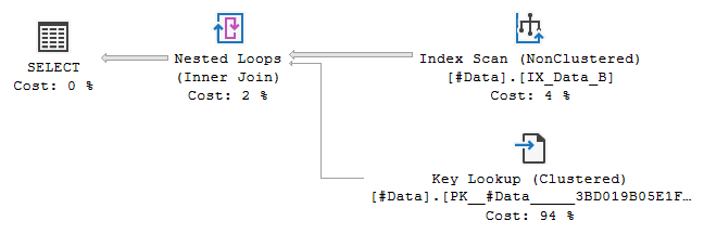
it can be forced with `INDEX` hint
```sql
SELECT [K]
FROM [#Data] WITH(INDEX([IX_Data_B]))
WHERE [A] = 2;
```
Estimated cost of this alternative execution plan encompasses cost of the Index Scan. Cost of the Index Scan itself can be less, equal or higher than cost of the plain Clustered Index Scan. If it is equal or higher, then there is no chance that entire plan cost can be lower than cost of Clustered Index Scan, and so consideration of the alternative would be knowingly losing.
During optimization, however, storage statistics comparison is performed earlier than cost calculation. One may object that comparison of storage statistics is not the same as comparison of costs. This is true, but, given the other influencing factors equal, it may be equivalent.
The above logic sounds plausible, but one flaw stemming from optimization path analysis haunts me.
## **Optimization Path**
I traced optimization paths for both the trivial and the full optimization cases to check optimization level choice logic, and also because of I was curious to know at what point storage statistics check happens.
### Trivial Optimization
Following is how trivial optimization for the subject query goes. Right before trivial optimization is entered, the logical tree of the query looks as
```none
*** Tree After Project Normalization ***
LogOp_Select
LogOp_Get TBL: #Data #Data TableID=-1182085811 TableReferenceID=0 IsRow: COL: IsBaseRow1000
ScaOp_Comp x_cmpEq
ScaOp_Identifier QCOL: [tempdb].[dbo].[#Data].A
ScaOp_Const TI(int,ML=4) XVAR(int,Not Owned,Value=2)
****************************************
```
(trace flag 8606 can be used to obtain it).
Once trivial optimization is entered, the `SelToTrivialFilter` rule is applied first, it makes call to index matching logic. Storage statistics are checked as a part of this logic. Necessary conditions are met, that causes the `SelToTrivialFilter` rule to produce its result. The query tree becomes
```none
***** Rule applied: Sel Table -> Index expression (SelToTrivialFilter)
PhyOp_NOP
LogOp_SelectRes
LogOp_GetIdx TBL: #Data TableID=-1182085811 index 1
ScaOp_Comp x_cmpEq
ScaOp_Identifier QCOL: [tempdb].[dbo].[#Data].A
ScaOp_Const TI(int,ML=4) XVAR(int,Not Owned,Value=2)
```
The `LogOp_SelectRes` (residual predicate) does not suppose any further actions except physical implementation, unlike the `LogOp_Select`, which can be simplified and explored also (not during trivial optimization though). Similarly, the `LogOp_GetIdx` denotes that specific index has been chosen and physical implementation should follow.
Then, the `SelResToFilter` rule implements `LogOp_SelectRes` as `PhyOp_Filter`, and the `GetIdxToRng` rule implements `LogOp_GetIdx` as `PhyOp_Range`. The result, in the end, is the physical tree produced
```none
*** Output Tree: (trivial plan) ***
PhyOp_NOP
PhyOp_Filter
PhyOp_Range TBL: #Data(1) ASC Bmk ( QCOL: [tempdb].[dbo].[#Data].K) IsRow: COL: IsBaseRow1000
ScaOp_Comp x_cmpEq
ScaOp_Identifier QCOL: [tempdb].[dbo].[#Data].A
ScaOp_Const TI(int,ML=4) XVAR(int,Not Owned,Value=2)
********************
```
(one can use trace flag 8607 to see it).
### Full Optimization
Beginning of the optimization path is identical for the full optimization case. Differences start at trivial optimization attempt, where the `SelToTrivialFilter` rule is applied, but fails because of conditions required by index matching logic are not met. Trivial optimization exits early and optimizer proceeds with full optimization.
Plan search goes very shortly, these are the only rules applied
```none
---------------------------------------------------
Apply Rule: SelectToFilter - Select()->Filter()
---------------------------------------------------
Apply Rule: GetToScan - Get()->Scan()
---------------------------------------------------
Apply Rule: GetToIdxScan - Get -> IdxScan
```
(trace flag 8619 can be used to get the list).
Most important to note here is that there are no signs of consideration of Index Scan with Key Lookup alternative (neither among the rules applied nor in the final memo structure).
Assuming that logic formulated in The Logic Behind section is correct, the situation looks paradoxical. Trivial optimization fails, because of it accounts for the alternative that should be considered during full optimization. Full optimization starts, but this alternative is not only not chosen, it is not considered even. This looks like a mistake to me. Either full optimization should not be triggered in this case without index hint in place, or logic behind is different.
After plan search is completed, the physical tree is produced
```none
*** Output Tree: ***
PhyOp_Filter
PhyOp_Range TBL: #Data(1) ASC Bmk ( QCOL: [tempdb].[dbo].[#Data].K) IsRow: COL: IsBaseRow1000
ScaOp_Comp x_cmpEq
ScaOp_Identifier QCOL: [tempdb].[dbo].[#Data].A
ScaOp_Const TI(int,ML=4) XVAR(int,Not Owned,Value=2)
********************
```
In this case it is almost identical to the one seen in the end of trivial optimization.
## **Other Factors Do Matter**
As a short sum up of previous sections, decision on "trivial vs full" optimization can depend on index matching logic, which in its turn can depend on storage statistics. Index matching logic, as one may anticipate, is more sophisticated and takes into account more factors.
As an example of additional factor, consider the following query
```sql
SELECT [K]
FROM [#Data]
WHERE [A] = 2 AND [B] IS NOT NULL;
```
The index `IX_Data_B` is non-covering for this query, and after fill-factor change it has the same number of leaf-level pages as the clustered index. These were the suitable conditions for the query considered earlier to qualify for trivial optimization. This query demands full optimization however, because of part of the `WHERE` predicate matches existing index key, which presents opportunity for index strategy.
The other example is that with index added
```sql
CREATE INDEX [IX_Data_C] ON [#Data] ([C]);
```
first query will no longer qualify for trivial optimization, because of now there is the other index with number of leaf-level pages less than clustered index has
| index_id | index_name | index_type_desc | index_depth | index_level | page_count | record_count |
| --------:| ---------- | --------------- | -----------:| -----------:| ----------:| ------------:|
| 1 | PK_#Data_3BD019B05E1F9831 | CLUSTERED INDEX | 2 | 0 | 5 | 1001 |
| 1 | PK_#Data_3BD019B05E1F9831 | CLUSTERED INDEX | 2 | 1 | 1 | 5 |
| 2 | IX_Data_B | NONCLUSTERED INDEX | 2 | 0 | 5 | 1001 |
| 2 | IX_Data_B | NONCLUSTERED INDEX | 2 | 1 | 1 | 5 |
| 3 | IX_Data_C | NONCLUSTERED INDEX | 2 | 0 | 4 | 1001 |
| 3 | IX_Data_C | NONCLUSTERED INDEX | 2 | 1 | 1 | 4 |
These are just some examples, without pretending to be a comprehensive analysis. There may be other factors of course.
## **Summary**
It is reasonable to expect that choice of the optimization level (trivial or full) for a query depends on query pattern or meta-information (tables and indexes definitions). It is possible, however, for the optimization level to be different without changing any of these, depending on just data. Simple `SELECT` with predicate from a table is the example particularly, if none of the existing indexes are covering for the query and none of them are useful with respect to predicate evaluation.
[^1]: [Query Optimizer Deep Dive](https://www.sql.kiwi/2012/04/query-optimizer-deep-dive-part-1.html) by Paul White
[^2]: [When does a Query Get Trivial Optimization?](https://www.brentozar.com/archive/2015/06/when-does-a-query-get-trivial-optimization/) by Kendra Little
[^3]: [What’s The Point of 1 = (SELECT 1)?](https://www.erikdarlingdata.com/sql-server/whats-the-point-of-1-select-1/) by Erik Darling
[4]: https://www.erikdarlingdata.com/sql-server/whats-the-point-of-1-select-1/